Note: This example is available as an interactive Jupyter notebook in the file Notebooks/Tutorial2.ipynb

Tutorial 2: Simulating survey datasets

In this tutorial, we will review how to use the Survey class to simulate an exoplanet survey, as well as how to configure the Survey’s parameters.

Setup

Let’s start by importing the necessary module from Bioverse.

# Import numpy
import numpy as np

# Import the Generator, ImagingSurvey, and TransitSurvey classes
from bioverse.generator import Generator
from bioverse.survey import ImagingSurvey, TransitSurvey,read_scaling_dict, prioritize_survey

# Import pyplot (for making plots later) and adjust some of its settings
from matplotlib import pyplot as plt
%matplotlib inline
plt.rcParams['font.size'] = 20.

Loading the Survey object

Bioverse uses ImagingSurvey and TransitSurvey objects to simulate datasets from a direct imaging or transit spectroscopy exoplanet survey. Each has a ‘default’ option. Let’s take a look at the default imaging survey:

# Load the 'defalt' imaging survey
survey = ImagingSurvey('default')

# Display some key properties
print("Telescope diameter: {:.1f} meters".format(survey.diameter))
print("Inner working angle: {:.1f} lambda/D".format(survey.inner_working_angle))
print("Outer working angle: {:.1f} lambda/D".format(survey.outer_working_angle))
print("Faintest detectable contrast: {:.1E}".format(10**survey.contrast_limit))

Telescope diameter: 15.0 meters
Inner working angle: 3.5 lambda/D
Outer working angle: 64.0 lambda/D
Faintest detectable contrast: 2.5E-11

Next, the default transit survey:

# Load the transit survey
survey = TransitSurvey('default')

# Display some key properties
print("Effective telescope diameter: {:.1f} meters".format(survey.diameter))
print("Maximum survey lifetime: {:.1f} years".format(survey.t_max/365.25))

Effective telescope diameter: 50.0 meters
Maximum survey lifetime: 10.0 years

Each survey is capable of conducting a set of measurements on the planets it observes. Let’s take a look at the transit survey:

print(survey)

TransitSurvey with the following parameters:
  label: default
  diameter: 50.0
  t_max: 3652.5
  t_slew: 0.0208
  N_obs_max: 1000
  mode: transit
  d_max: nan
  P_max: nan
  min_depth: nan
  m_G_max: nan

Conducts the following measurements
(0) Measures parameter 'L_st'
(1) Measures parameter 'R_st' with 5% precision
(2) Measures parameter 'M_st' with 5% precision
(3) Measures parameter 'T_eff_st' with 25.0 precision
(4) Measures parameter 'd'
(5) Measures parameter 'H'
(6) Measures parameter 'age' with 30% precision
(7) Measures parameter 'depth'
(8) Measures parameter 'T_dur'
(9) Measures parameter 'P' with 0.001 precision
(10) Measures parameter 'EEC'

Each measurement is conducted in the order it is listed. Some have values are measured with approximately zero uncertainty (e.g. distance to the star), while others are measured with poorer precision (e.g. +- 30% for the system’s age).

Producing simulated datasets

The first step in a simulated Survey is to determine which simulated planets can actually be detected. Let’s start by generating a sample of planets orbiting stars that might be targeted by LUVOIR.

# Generate a sample of planetary systems
generator = Generator('imaging')
sample = generator.generate()

Next, we use the imaging Survey object to determine which of these planets can be detected by LUVOIR.

survey = ImagingSurvey('default')
detected = survey.compute_yield(sample)

print("Detected {:d} planets including {:d} exo-Earth candidates.".format(len(detected), detected['EEC'].sum()))

Detected 330 planets including 19 exo-Earth candidates.

Finally, we simulate a dataset from observations of all of the detected planets over the course of 10 years.

data = survey.observe(detected, t_total=10*365.25)

The values in data are imprecise measurements of the true values in detected. For example, let’s look at the fractional measurement error on the semi-major axis.

error = (data['a']-detected['a'])/detected['a']
std = np.std(error)

plt.hist(error*100, bins=10)
plt.xlabel('% error on semi-major axis')
plt.axvline(-std, c='black', lw=5, linestyle='dashed')
plt.axvline(std, c='black', lw=5, linestyle='dashed')
plt.show()

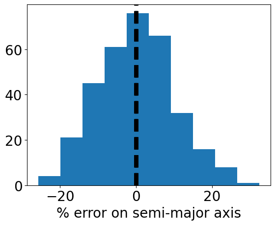
The standard deviation, highlighted by black lines, is about 10%. This is the estimated uncertainty in semi-major axis determination following ~3 direct imaging revisits (Guimond & Cowan 2019).

Let’s repeat this exercise for the transit survey. This time we will use the stellar mass function to generate host stars, and the quickrun() function to consolidate the steps.

# Load the Generator and Survey
generator = Generator('transit')
survey = TransitSurvey('default')

# Instead of this:
# sample = generator.generate(transit_mode=True)
# detected = survey.compute_yield(generator)
# data = survey.observe(sample, t_total=10*365.25)

# Use this:
sample, detected, data = survey.quickrun(generator, t_total=10*365.25) # note that transit_mode = True is automatically passed for transit surveys

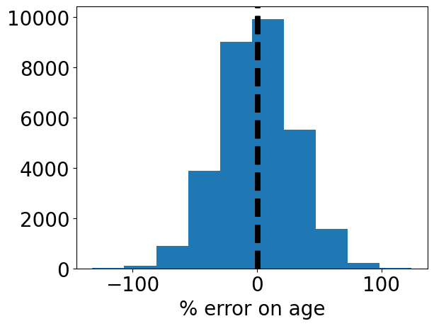
Because the transit survey mostly observes low-mass stars, planet ages are difficult to constrain. The state of the art for low-mass stellar age constraints is around 30% (for TRAPPIST-1; see Burgasser & Mamajek 2017)

error = (data['age']-detected['age'])/detected['age']
std = np.std(error)

plt.hist(error*100, bins=10)
plt.xlabel('% error on age')
plt.axvline(-std, c='black', lw=5, linestyle='dashed')
plt.axvline(std, c='black', lw=5, linestyle='dashed')
plt.show()

Time constraints

In principle, the transit survey is capable of detecting and characterizing any transiting planet, provided it can observe enough transits to build up the spectroscopic signal-to-noise ratio. In reality, the total number of transits it can observe is limited by survey duration.

For example, a key observable parameter for terrestrial planets is the presence (or absence) of H2O in the atmosphere. However, water clouds obscure almost all absorption from water vapor along the same sightlines. Using the Planetary Spectrum Generator with sophisticated GCM models that include the effects of clouds, we have estimated that the transit survey will require approximately ~7.5 days of in-transit observing time for a typical star, assuming a 50-meter effective diameter. We incorporate this assumption into the ‘has_H2O’ measurement:

#import dictionary with reference times
scaling_dict=read_scaling_dict("transit_H2O")
#set those reference times to be used in the exposure time calculation
survey.set_reference_observation(**scaling_dict)

prioritize_survey(survey,'transit_H2O')

#add H2O measurement to survey measurements
survey.add_measurement('has_H2O')

# Retrieve the time required for the has_H2O measurement
t_ref = scaling_dict['t_ref']

# Properties of the reference star
T_st_ref = scaling_dict['T_st_ref']
R_st_ref = scaling_dict['R_st_ref']

print("Reference star properties: R = {:.1f} R_sun and T_eff = {:.0f} K".format(R_st_ref, T_st_ref))
print("Time required to characterize an Earth-like planet around this star: {:.1f} d".format(t_ref))

Reference star properties: R = 0.3 R_sun and T_eff = 3300 K
Time required to characterize an Earth-like planet around this star: 7.5 d

t_ref is scaled according to planet size, stellar size, stellar distance, atmospheric scale height, etc. to produce an estimate for the observing time required for each individual planet.

Rerun bioverse to include the exposure time dependent observation

sample = generator.generate()
#to account for the exposure time required per observation, and to calculate that exposure time
#with a scaling relation set the method in the yield calculation to 'scaling_relation'
detected= survey.compute_yield(sample,method='scaling_relation')
data = survey.observe(detected)

#to return all detectable planets set method='detectable'
all_detectable= survey.compute_yield(sample,method='detectable')
#to see what exposure times are for non selected targets call the exp_time_scaling_relation function
#normally called within the compute_yield function
all_detectable = survey.exp_time_scaling_relation(all_detectable)

#get exposure time and number of transits for exoEarths
is_EEC= (all_detectable['EEC']==True)
detectable_eecs=all_detectable[is_EEC]
t_exp= detectable_eecs['t_exp']
N_obs= detectable_eecs['N_obs']

Plotted below are the exposure times (and number of transit observations) required to find H2O in the atmospheres of transiting EECs. The dashed lines indicate a generous upper limit of 1,000 combined transit observations of ~1 hr duration.

fig, ax = plt.subplots(ncols=2, figsize=(16,8))

bins = np.logspace(np.log10(0.01), np.log10(np.amax(t_exp)), 30)
ax[0].hist(t_exp, bins=bins)
ax[0].set_xscale('log')
ax[0].set_xlabel('Exposure time (d)')
ax[0].set_ylabel('Number of EECs')
ax[0].axvline(1000/24, linestyle='dashed', lw=5, c='black')

bins = np.logspace(0, 5, 30)
ax[1].hist(N_obs, bins=bins)
ax[1].set_xscale('log')
ax[1].set_xlabel('Number of transit observations')
ax[1].axvline(survey.N_obs_max, linestyle='dashed', lw=5, c='black')

plt.subplots_adjust(wspace=0.3)
plt.show()

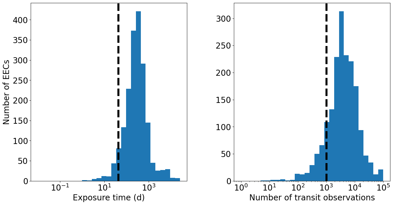
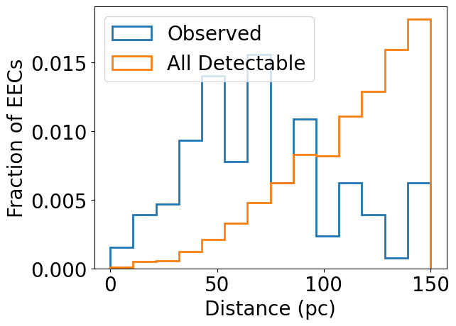
As a result, most exo-Earth candidates cannot be observed during the survey. Since the required exposure time scales with distance^2, the successfully observed targets tend to be much closer to Earth.

# Determines which EECs were observed vs not observed for atmospheric H2O
obs = ~np.isnan(data['has_H2O'])
EEC = detected['EEC']

bins = np.linspace(0, 150, 15)
plt.hist(data['d'][EEC], density=True, histtype='step', lw=2, bins=bins, label='Observed')
plt.hist(detectable_eecs['d'], density=True, histtype='step', lw=2, bins=bins, label='All Detectable')
plt.xlabel('Distance (pc)')
plt.ylabel('Fraction of EECs')
plt.legend(loc='upper left')

plt.show()

If we choose more optimistic assumptions about cloud cover, we can reduce t_ref and therefore increase the number of observable EECs:

t_ref = np.arange(1, 16)
N_EEC = np.zeros(len(t_ref))
for i, tr in enumerate(t_ref):
    survey.set_reference_observation(t_ref=tr)
    sample, detected, data = survey.quickrun(generator,method='scaling_relation', t_total=10*365.25)
    EEC = detected['EEC']
    N_EEC[i] = np.sum(~np.isnan(data['has_H2O'][EEC]))

plt.plot(t_ref, N_EEC, lw=3)
plt.xlim([0, 15])
plt.xlabel('Avg time required per target (d)')
plt.ylabel('Number of EECs\ncharacterized')

plt.show()

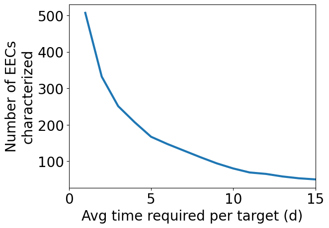
Note that these exposure time considerations apply equally to imaging surveys. However, given low values of eta Earth assumed (~7.5%), even a LUVOIR-like survey will likely be volume-limited in the number of EECs it can characterize. For a given observatory configuration, the number of EECs it can spectroscopically characterize is mostly a function of eta Earth. For highly time-intensive observations (e.g. rotational mapping), this may not be the case.