Computing statistical power
Consider the “habitable zone hypothesis”, which proposes that habitable planets with atmospheric water vapor will be more common within the semi-major axis range a_inner < a_eff < a_outer (see Section 6 of the paper and Example 1 for more details). In Bioverse, this effect is injected into the simulated sample by the Example1_water() function, and tested using the h_HZ Hypothesis. To test this hypothesis using a LUVOIR-like direct imaging survey:
from bioverse.generator import Generator
from bioverse.survey import ImagingSurvey
from bioverse.hypothesis import h_HZ

# Load the Generator and Survey objects
generator = Generator('imaging')
survey = ImagingSurvey('default')

# Generate a set of planetary systems and a simulated dataset as observed by an imaging survey
# Assume 50% of EECs are habitable (f_water_habitable=0.5)
# Assume 1% of non-habitable planets have water vapor (f_water_nonhabitable=0.01)
sample, detected, data = survey.quickrun(generator, f_water_habitable=0.5, f_water_nonhabitable=0.01)

# Test the habitable zone hypothesis from this dataset
results = h_HZ.fit(data)

print("The evidence in favor of the habitable zone hypothesis is {:.1f}.".format(results['dlnZ']))
Output: The evidence in favor of the habitable zone hypothesis is 6.4.
This result corresponds to a “p-value” of ~1.7E-3. However, this represents only one possible realization of the survey. Due to Poisson uncertainty, another equivalent survey might detect fewer habitable planets and thus be less capable of testing the hypothesis. To capture this, we can repeat the survey several times and average their results. The analysis module enables this through its test_hypothesis_grid() function.
from bioverse import analysis

# Repeat the hypothesis test N=30 times with the same assumptions as above
results = analysis.test_hypothesis_grid(h_HZ, generator, survey, N=30, f_water_habitable=0.5,
                                        f_water_nonhabitable=0.01, processes=8)

# Determine the statistical power assuming a significance threshold of dlnZ > 3
power = analysis.compute_statistical_power(results, method='dlnZ', threshold=3)

print("The statistical power of the survey is {:.1f}%".format(100*power))
Output: The statistical power of the survey is 75.0%.
Under the assumptions that 50% of exo-Earth candidates are habitable and 1% of non-habitable planets have H2O in their atmospheres, it is 75% likely that a LUVOIR-like survey would be able to detect the overabundance of H2O in the habitable zone.
Parameter grids
Of course, those assumptions are highly uncertain, and a more thorough analysis should investigate how this result depends on key model parameters - such as f_water_habitable or eta_Earth. This can be done by passing an array of values for these parameters to the test_hypothesis_grid() function:
# Vary the fraction of EECs with water vapor from 1% to 100% (log spacing)
f_water_habitable = np.logspace(-2, 0, 5)

# Vary eta Earth from 7.5% to 30% (linear spacing)
eta_Earth = np.linspace(0.075, 0.3, 5)

# Test the hypothesis N=30 times for each parameter combination
results = analysis.test_hypothesis_grid(h_HZ, generator, survey, N=30, f_water_habitable=f_water_habitable,
                                        eta_Earth=eta_Earth, f_water_nonhabitable=0.01, processes=8)

# Compute the statistical power for each parameter combination
power = analysis.compute_statistical_power(results, method='dlnZ', threshold=3)
power will be a 5x5 array containing the statistical power for each parameter combination. The axis order depends on the order in which arguments are passed to test_hypothesis_grid(); in this case, f_water_habitable will correspond to the first axis and eta_Earth to the second.
Plotting the results
The plot_power_grid() function can be used to plot the statistical power over a 2-dimensional grid. Starting from the above example:
from bioverse.plots import plot_power_grid

# Specify which parameters to plot on the x and y axes
axes = ('f_water_habitable', 'eta_Earth')

# Set the axis labels
labels = ('Fraction of EECs that are habitable', 'eta Earth')

# Set log-scale for the x axis
log = (True, False)

# Create the plot
plot_power_grid(results, axes=axes, labels=labels, log=log)
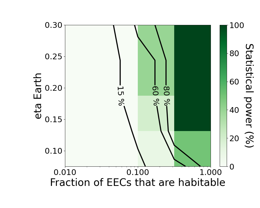
The number and percentage values of the contour lines can be set with the levels argument, or set levels=None to disable them. To create a higher resolution plot with smoother contour lines, simply run test_hypothesis_grid() over a finer grid of parameter values.
Multiprocessing
To compute the statistical power for a 20x20 parameter grid with N=50 simulations in each cell requires 20,000 simulations, or approximately 5-6 hours for the example above. Fortunately, these simulations are entirely independent of each other, making parallel processing an effective solution. You can use the processes argument of test_hypothesis_grid() to indicate how many processes to run in parallel. Note that Bioverse can be memory-intensive, so large values of processes (e.g. greater than 10) can have diminishing returns or lead to a crash.